课程[链接](https: // www.youtube.com / watch?v = c36lUUr864M)
1. Tensor
1.1 How to create tensor
构造tensor的方法主要有六种,分别如下:
x = torch.ones(3, 5, dtype=torch.float, requires_grad = True )
x = torch.zeros(3, 5, dtype=torch.float, requires_grad = True )
x = torch.rand(3, 5, dtype=torch.float, requires_grad = True )
x = torch.empty(3, 5, dtype=torch.float, requires_grad = True )
x = torch.tensor([1,2,3], dtype=torch.float, requires_grad = True )
x_numpy = np.array([1,2,3])
x = torch.from_numpy(x_numpy)
1.2 对Tensor的各种操作
查看数据类型:x.dtype
查看size:x.size()
如果tensor只有一个值,查看实数值:x.item()
改变tensor的形状大小:x = x.view(num_row, num_col)
将tensor转为numpy: z = x.detach().numpy()
注意:numpy只能存放到cpu上面,并且不能是包含梯度的tensor,转换之后共享相同的内存
- 构造新的不包含梯度的tensor:z = x.detach()
- 对tensor进行各种转换: .to() eg: x.to(int)
1.3 基本运算
- add: z = x+y
- minus: z = x-y
- multi: z = x*y
- div: z = x/y
- 切片操作:切片操作十分灵活,用到的时候查询文档
2. Autograd
2.1 Calculate the gradients
用 z.backward() 来计算z关于变量的梯度,如果正向计算出来的z是一个实数值,则backward的参数为默认值就好,如果z是一个向量,则调用backward()的时候需要传入一个与z的size相同的向量.
如下面的示例所示。
2
3
4
5
6
7
8
9
10
11
12
13
y=x*x+2*x+5
z = torch.mean(y)
z.backward() # dz/dx jacobian matrix to get the grad
# z.backward()这一步是用雅可比矩阵来计算梯度,如果正向计算出来的z是
# 一个实数值,则backward的参数为默认值就好,如果z是一个向量,则调用
# backward()的时候需要传入一个与z的size相同的向量
#
# y = x*x*2+x
# v = torch.tensor([1.00,0.10,0.200], dtype=torch.float32)
# y.backward(v)
#
print(x.grad)
2.2 How to prevent pytorch from tracking the history and calculating this grad fn attribute.
一共有三种方法让tensor不被计算图追踪梯度,分别是:
1) x.requires_grad_(False)
2) x.detach()
3) with torch.no_grad(): pass
具体示例如下所示:
2
3
4
5
6
7
8
9
10
11
print(x)
# 让张量x不在追踪梯度的方法有三种
# x.requires_grad_(False)
# x.detach()
# with torch.no_grad():
with torch.no_grad():
y = x+2
print(x) # x with grad
print(y) # y without grad
2.3 梯度累积
调用backward()来计算梯度的时候,当前轮次的梯度,是之前所有轮次梯度的累积和,在梯度下降学习中这是我们不想看到的,可以调用zero_()函数来将梯度变为0.
示例如下:
2
3
4
5
6
7
8
9
10
11
12
13
14
for epoch in range(2):
model_output = (weights*3).sum()
model_output.backward()
print(weights.grad)
# weights.grad.zero_()
# 输出结果为:
# tensor([3., 3., 3.])
# tensor([6., 6., 6.])
# 第一个epoch为3,第二个epoch为6,说明梯度在累加
# 因为梯度累积是我们不希望看到的,所以每次迭代的时候我们希望梯度
# 能够清零,梯度清零用.grad.zero_()函数
3. Backpropagation
调用backward()函数来进行反向传播,计算梯度,示例如下:
2
3
4
5
6
7
8
9
10
11
12
13
14
y = torch.tensor(2, dtype=torch.float32, requires_grad=False)
w = torch.tensor(1, dtype=torch.float32, requires_grad=True)
loss = (x*w-y)**2
print(loss)
loss.backward()
print(w.grad)
## output:
# tensor(1., grad_fn=<PowBackward0>)
# tensor(-2.)
4. Optimize model with automatic gradient computation
4.1 用numpy实现回归算法
实现回归算法分为如下几步:
1) 数据准备
2)定义function
3)定义loss function
4) 定义梯度计算公式
5) 编写training loop部分代码
实现代码如下:
2
3
4
5
6
7
8
9
10
11
12
13
14
15
16
17
18
19
20
21
22
23
24
25
26
27
28
29
30
31
32
33
34
35
36
37
# f = 2 * x
# 1. 用numpy手动实现
# prepare dataset
X = np.array([1,2,3,4,5,6,7], dtype=np.float32)
y = np.array([2,4,6,8,9,13,20], dtype=np.float32)
w = 0.0
# model prediction
def forward(x):
return w*x
# loss = MSE
def loss(y, y_pred):
return ((y_pred - y)**2).mean()
# gradient
def gradient(x,y,y_pred):
return (2*x*(y_pred - y)).mean()
print(f'Prediction before training: f(5) = {forward(5):.5f}')
# Training
learning_rate = 0.1
n_iters = 10
for i in range(n_iters):
y_pred = forward(X)
l = loss(y, y_pred)
dw = gradient(x, y, y_pred)
w -= learning_rate*dw
print(f'epoch {i+1}: w = {w:.3f}, loss = {l:.10f}')
print(f'Prediction after training: f(5) = {forward(5):.5f}')
4.2 用pytorch替换数据类型和梯度计算
代码实现思路与4.1一样,没有做任何变化。
示例代码如下:
2
3
4
5
6
7
8
9
10
11
12
13
14
15
16
17
18
19
20
21
22
23
24
25
26
27
28
29
30
31
32
33
34
35
36
X = torch.tensor([1,2,3,4,5,6,10], dtype=torch.float32)
y = torch.tensor([2,4,6,8,10,12,20], dtype=torch.float32)
w = torch.tensor(0.0, dtype=torch.float32, requires_grad = True)
# model prediction
def forward(x):
return w*x
# loss = MSE
def loss(y, y_pred):
return ((y_pred - y)**2).mean()
print(f'Prediction before training: f(5) = {forward(5):.5f}')
# Training
learning_rate = 0.0001
n_iters = 10000
for i in range(n_iters):
y_pred = forward(X)
l = loss(y, y_pred)
l.backward()
with torch.no_grad():
w -= learning_rate*w.grad
w.grad.zero_()
if (i+1) %1000 == 0:
print(f'epoch {i+1}: w = {w:.3f}, loss = {l:.10f}')
print(f'Prediction after training: f(5) = {forward(5):.5f}')
4.3 用pytorch来做梯度计算和优化
4.2 我们用了backward()函数来自动计算梯度,但是梯度下降优化算法依然是我们在4.1版本中的手工编写的公式,这里我们在之前的基础上面更进一步,用pytorch框架中的optimizer来替换掉手工编写的梯度下降方法,代码如下:
2
3
4
5
6
7
8
9
10
11
12
13
14
15
16
17
18
19
20
21
22
23
24
25
26
27
28
29
30
31
32
33
34
35
36
37
38
39
40
41
42
43
44
45
46
47
# 2) Construct loss and optimizer
# 3) Training loop
# - forward pass: compute prediction
# - backward pass: gradients
# - update weight
import torch.nn as nn
X = torch.tensor([[1],[2],[3],[4],[5],[6],[10]], dtype=torch.float32)
y = torch.tensor([[2],[4],[6],[8],[10],[12],[20]], dtype=torch.float32)
x_test = torch.tensor([5], dtype=torch.float32)
n_samples, n_features = X.shape
print(n_samples, n_features)
input_size = n_features
output_size = n_features
model = nn.Linear(input_size, output_size)
print(f'Prediction before training: f(5) = {model(x_test).item():.5f}')
# Training
learning_rate = 0.01
n_iters = 1000
loss = nn.MSELoss()
optimizer = torch.optim.SGD(model.parameters(), lr=learning_rate)
for i in range(n_iters):
y_pred = model(X)
l = loss(y, y_pred)
l.backward()
optimizer.step()
# w.grad.zero_()
optimizer.zero_grad()
if (i+1) %1000 == 0:
[w, b] = model.parameters()
print(f'epoch {i+1}: w = {w[0][0].item():.3f}, loss = {l:.10f}')
print(f'Prediction after training: f(5) = {model(x_test).item():.5f}')
4.4 定义更加复杂的模型
4.3 及其之前的工作,我们对model的定义都及其的简单,这里我们对model进行改进,通过自定义一个LinearRegress对象来定义一个包含两层全连接的网络建模我们的model,隐藏层的激活函数我们选用了relu()激活函数。代码如下:
2
3
4
5
6
7
8
9
10
11
12
13
14
15
16
17
18
19
20
21
22
23
24
25
26
27
28
29
30
31
32
33
34
35
36
37
38
39
40
41
42
43
44
45
46
47
48
49
50
51
52
53
54
55
56
57
58
59
60
61
62
63
64
65
66
67
68
# 2) Construct loss and optimizer
# 3) Training loop
# - forward pass: compute prediction
# - backward pass: gradients
# - update weight
import torch.nn as nn
X = torch.tensor([[1],[2],[3],[4],[5],[6],[10]], dtype=torch.float32)
y = torch.tensor([[2],[4],[6],[8],[10],[12],[20]], dtype=torch.float32)
x_test = torch.tensor([5], dtype=torch.float32)
n_samples, n_features = X.shape
print(n_samples, n_features)
input_size = n_features
output_size = n_features
# model = nn.Linear(input_size, output_size)
class LinearRegress(nn.Module):
def __init__(self, input_size, output_size):
super(LinearRegress, self).__init__()
# define layers
self.lin1 = nn.Linear(input_size, 2)
self.lin2 = nn.Linear(2, output_size)
def forward(self, x):
x = self.lin1(x)
x = torch.relu(x)
return self.lin2(x)
model = LinearRegress(input_size, output_size)
print(f'Prediction before training: f(5) = {model(x_test).item():.5f}')
# Training
learning_rate = 0.01
n_iters = 1000
loss = nn.MSELoss()
optimizer = torch.optim.SGD(model.parameters(), lr=learning_rate)
for i in range(n_iters):
y_pred = model(X)
l = loss(y, y_pred)
l.backward()
optimizer.step()
# w.grad.zero_()
optimizer.zero_grad()
if (i+1) %1000 == 0:
# [w, b] = model.parameters()
# print(f'epoch {i+1}: parameters = {model.parameters()}, loss = {l:.10f}')
for parameters in model.parameters():
print(parameters)
print(f'Prediction after training: f(5) = {model(x_test).item():.5f}')
# Now pytorch can do most of the work for us, of course we still have to design our model
# and have to know which loss and optimizer we want to use but we don't have to worry about
# the underlying algorithms anymore.
4.5 综合示例1
学习完了4.1-4.3的内容,我们对如何手工建模一个模型有了初步的了解,并且知道了pytorch建模深度学习的一般过程,以及它对应的每一个部分的作用,下面我们通过一个综合的示例来加深对所学知识的理解。
在该示例中,我们首先调用sklearn的datasets库来构建带噪声的逻辑回归数据集,然后构造一个线性模型,并对线性模型进行训练。代码如下:
2
3
4
5
6
7
8
9
10
11
12
13
14
15
16
17
18
19
20
21
22
23
24
25
26
27
28
29
30
31
32
33
34
35
36
37
38
39
40
41
42
43
44
45
46
47
48
49
import torch
import torch.nn as nn
import numpy as np
from sklearn import datasets
import matplotlib.pyplot as plt
# 0) create data
x_numpy, y_numpy = datasets.make_regression(n_samples=500, n_features=1, noise=20, random_state=1)
x,y = torch.from_numpy(x_numpy.astype(np.float32)), torch.from_numpy(y_numpy.astype(np.float32))
# print(x.shape)
# print(y.shape)
y = y.view(y.shape[0], -1)
# print(y.shape)
n_sample, n_features = x.shape
# 1) model
input_size = n_features
output_size = 1
model = nn.Linear(input_size, output_size)
# 2)loss and optimizer
learning_rate = 0.01
criterion = nn.MSELoss()
optimizer = torch.optim.SGD(model.parameters(), lr=learning_rate)
# 3) training loop
num_epochs = 1000
num_iter = 100
for epoch in range(num_epochs):
# foreard pass and loss
y_pred = model(x)
loss = criterion(y_pred, y)
# backward pass
loss.backward()
# updata
optimizer.step()
optimizer.zero_grad()
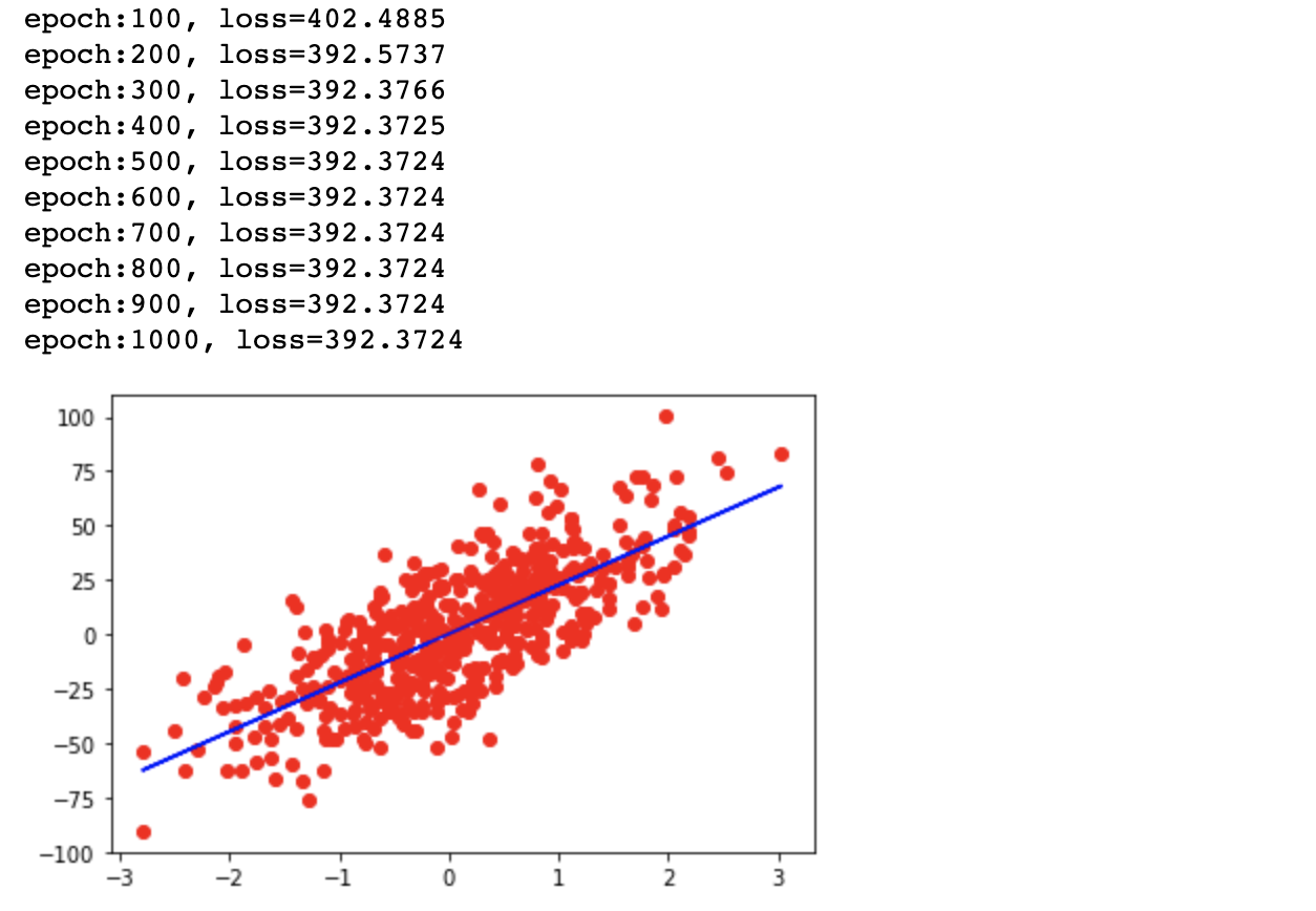
if(epoch+1)%num_iter == 0:
print(f'epoch:{epoch+1}, loss={loss.item():.4f}')
# plot
predicted = model(x).detach().numpy()
plt.plot(x_numpy, y_numpy, 'ro')
plt.plot(x_numpy, predicted, 'b')
plt.show()运行结果如下:
4.6 综合示例2
之前的示例中我们没有对训练后的模型进行测试,在这个例子中我们增加了模型测试,并且调用sklearn中内置的“乳腺癌”数据集来完成示例,并且对输入特征做了归一化处理。
代码如下:
2
3
4
5
6
7
8
9
10
11
12
13
14
15
16
17
18
19
20
21
22
23
24
25
26
27
28
29
30
31
32
33
34
35
36
37
38
39
40
41
42
43
44
45
46
47
48
49
50
51
52
53
54
55
56
57
58
59
60
61
62
63
64
65
66
67
68
69
70
71
72
73
74
import torch
import torch.nn as nn
import numpy as np
from sklearn import datasets
from sklearn.preprocessing import StandardScaler
from sklearn.model_selection import train_test_split
# 0) prepare data
bc = datasets.load_breast_cancer()
X,y = bc.data, bc.target
n_samples, n_features = X.shape
# print(X.shape)
# print(y.shape)
X_train, X_test, y_train, y_test = train_test_split(X,y,test_size=0.2, random_state=1234)
# scale 对每一列的特征做均值方差归一化处理,如果不做的话学习出来的模型的准确率大大降低
sc = StandardScaler()
# print('X_test before transform:', X_test)
X_train = sc.fit_transform(X_train)
X_test = sc.fit_transform(X_test)
# print('X_test after transform:', X_test.mean(), X_test.std())
X_train = torch.from_numpy(X_train.astype(np.float32))
X_test = torch.from_numpy(X_test.astype(np.float32))
y_train = torch.from_numpy(y_train.astype(np.float32))
y_test = torch.from_numpy(y_test.astype(np.float32))
y_train = y_train.view(y_train.shape[0], 1)
y_test = y_test.view(y_test.shape[0], 1)
# 1) model
# f = wx + b, sigmoid at the end
class LogisticRegression(nn.Module):
def __init__(self, n_input_features):
super(LogisticRegression, self).__init__()
self.linear = nn.Linear(n_input_features, 1)
def forward(self, x):
y_pred = torch.sigmoid(self.linear(x))
return y_pred
model = LogisticRegression(n_features)
# 2) loss and optimizer
learning_rate = 0.001
criterion = nn.BCELoss()
optimizer = torch.optim.SGD(model.parameters(), lr = learning_rate)
# 3) training loop
num_epochs = 1000
for epoch in range(num_epochs):
# foreard pass and loss
y_pred = model(X_train)
loss = criterion(y_pred, y_train)
# backward pass
loss.backward()
# updates
optimizer.step()
optimizer.zero_grad()
if(epoch+1) % 100 == 0:
print(f'epoch:{epoch+1}, loss = {loss.item():.4f}')
with torch.no_grad():
y_pred = model(X_test)
y_pred_cls = y_pred.round() # 对sigmoid出来的值进行四舍五入
# print(f'y_pred={y_pred}, y_pred_cls={y_pred_cls}')
acc = y_pred_cls.eq(y_test).sum()/float(y_test.shape[0])
print(f'acc = {acc:.4f}')
5. Dataset and Dataload Class
5.1 Dataset and Dataload
pytorch中由dataset类管理数据集,可以通过继承dataset类来自定义数据集,代码模板如下:
2
3
4
5
6
7
8
9
def __init__(self):
pass
def __getitem__(self, index):
return a signel data
def __len__(self):
return length of dataset定义好dataset之后,可以通过DataLoader来构造可供训练的迭代器,代码如下:
示例如下所示:
2
3
4
5
6
7
8
9
10
11
12
13
14
15
16
17
18
19
20
21
22
23
24
25
26
27
28
29
30
31
32
33
34
35
36
37
38
39
40
41
42
43
44
45
46
47
48
49
50
51
52
53
54
55
56
57
58
59
60
61
62
63
epoch = 1 forward and backward pass of ALL training samples
bach_size = number of training samples in one forward & backward pass
number of iterations = number of passes, each pass using [batch_size] number of samples
e.g. 100 samples, batch_size = 20 --> 100/20 = 5 iterations for 1 epoch
'''
import torch
import torchvision
from torch.utils.data import Dataset, DataLoader
import numpy as np
import math
import os
if not os.getcwd().endswith('pytorchLearning'):
os.chdir(os.getcwd()+'/Desktop/pytorchLearning')
# print (os.getcwd())
class WineDataset(Dataset):
def __init__(self):
# data loading
xy = np.loadtxt('./data/wine/wine.csv', delimiter=',', dtype=np.float32, skiprows=1)
self.x = torch.from_numpy(xy[:,1:])
self.y = torch.from_numpy(xy[:, [0]])
self.n_samples = xy.shape[0]
def __getitem__(self, index):
return self.x[index], self.y[index]
def __len__(self):
return self.n_samples
# # How we can use dataset
# dataset = WineDataset()
# first_data = dataset[0]
# features, label = first_data
# print(features, label)
#
# # How we can use dataload
# dataloader = DataLoader(dataset=dataset, batch_size=4, shuffle=True, num_workers=2)
#
# dataiter = iter(dataloader)
# data = dataiter.next()
# features, label = data
# print(features, label)
dataset = WineDataset()
dataloader = DataLoader(dataset=dataset, batch_size=4, shuffle=True, num_workers=2)
# training loop
num_epochs=2
total_samples = len(dataset)
n_iterations = math.ceil(total_samples/4)
print(total_samples, n_iterations)
for epoch in range(num_epochs):
for i,(inputs, label) in enumerate(dataloader):
# forward backward, update
if (i+1) % 5 == 0:
print(f'epoch {epoch+1}/{num_epochs}, step {i+1}/{n_iterations}, inputs {inputs.shape}')
5.2 Transforms for the dataset
pytorch通过传入transforms类来对输入的数据进行某种变化,transforms类可以调用库定义好的,也可以根据需要自定义。
示例代码如下:
2
3
4
5
6
7
8
9
10
11
12
13
14
15
16
17
18
19
20
21
22
23
24
25
26
27
28
29
30
31
32
33
34
35
36
37
38
39
40
41
42
43
44
45
46
47
48
49
50
51
52
53
54
55
56
57
58
59
60
61
62
63
64
65
66
67
68
69
70
71
72
73
74
75
76
77
78
79
80
81
82
83
84
85
86
87
88
89
90
91
92
93
Transforms can be applied to PIL images, tensor, ndarrays, or custom data
during criterion of the dataset
complete list of built-in transforms:
https://pytorch.org/docs/stable/torchvision/transforms.html
On images
---------
CenterCrop, Grayscale, Pad, RandomAffine,
RandomCrop, RandomHorizontalFlip, RandomHorizon
Resize, scale
On Tensors
----------
LinearTransformation, Normalize, RandomErasing
Conversion
----------
ToPILIamage: from tensor or ndarray
ToTensor: from numpy.ndarray or PILImage
Generic
-------
Use Lambda
Custom
------
Write own Class
Compose mutiple Transforms
--------------------------
composed = transforms.Compose([Rescale(256),
RandomCrop(224)])
torchvision.transforms.Rescale(256)
torchvision.transforms.ToTensor()
'''
import torch
import torchvision
from torch.utils.data import Dataset
import numpy as np
class WineDataset(Dataset):
def __init__(self, transform=None):
xy = np.loadtxt('./data/wine/wine.csv', delimiter=',', dtype=np.float32, skiprows=1)
self.n_samples = xy.shape[0]
# note that we do not convert to tensor here
self.x = xy[:,1:]
self.y = xy[:, [0]]
self.transform = transform
def __getitem__(self, index):
sample = self.x[index], self.y[index]
if self.transform:
sample = self.transform(sample)
return sample
def __len__(self):
return self.n_samples
class ToTensor:
def __call__(self, sample):
inputs, targets = sample
return torch.from_numpy(inputs), torch.from_numpy(targets)
class MulTransform:
def __init__(self, factor):
self.factor = factor
def __call__(self, sample):
inputs, target = sample
inputs *= self.factor
return inputs, target
dataset = WineDataset(transform=ToTensor())
first_data = dataset[0]
features, label = first_data
print(features)
print(type(features), type(label))
composed = torchvision.transforms.Compose([ToTensor(), MulTransform(2)]) # 把两个transforms合并一起应用
dataset = WineDataset(transform=composed)
first_data = dataset[0]
features, label = first_data
print(features)
print(type(features), type(label))
6. Softmax and Cross-Entropy
6.1 Softmax
1 | # Softmax |
6.2 Cross entropy
1 | # Cross entropy |
7. Activation function
Activation functions apply a non-linear transform and decide whether a neural should be activated or not.
Most popular activation functions
- Step function –> Not used in practice
- Sigmoid
- TanH
- ReLU
- Leaky ReLU
- Softmax
8. 综合练习 MNIST
MNIST
DataLoader, Transformation
Multilayer Neural Net, activation function
Loss and Optimizer
Tra
代码如下:
2
3
4
5
6
7
8
9
10
11
12
13
14
15
16
17
18
19
20
21
22
23
24
25
26
27
28
29
30
31
32
33
34
35
36
37
38
39
40
41
42
43
44
45
46
47
48
49
50
51
52
53
54
55
56
57
58
59
60
61
62
63
64
65
66
67
68
69
70
71
72
73
74
75
76
77
78
79
80
81
82
83
84
85
86
87
88
89
90
91
92
93
94
95
import torch.nn as nn
import torchvision
import torchvision.transforms as transforms
import matplotlib.pyplot as plt
import torch.nn.functional as F
import math
# device config
from torch.optim import optimizer
device =torch.device('cuda' if torch.cuda.is_available() else 'cpu')
# hyper parameters
input_size = 784 # 28x28
hidden_size = 128
num_classes = 10
num_epochs = 2
batch_size = 100
learning_rate = 0.001
# MNIST DataSet
train_dataset = torchvision.datasets.MNIST(root='./data', train=True,
transform=transforms.ToTensor(),download=True)
test_dataset = torchvision.datasets.MNIST(root='./data', train=False,
transform=transforms.ToTensor())
train_loader = torch.utils.data.DataLoader(dataset=train_dataset,batch_size=batch_size,
shuffle=True)
test_loader = torch.utils.data.DataLoader(dataset=test_dataset,batch_size=batch_size,
shuffle=False)
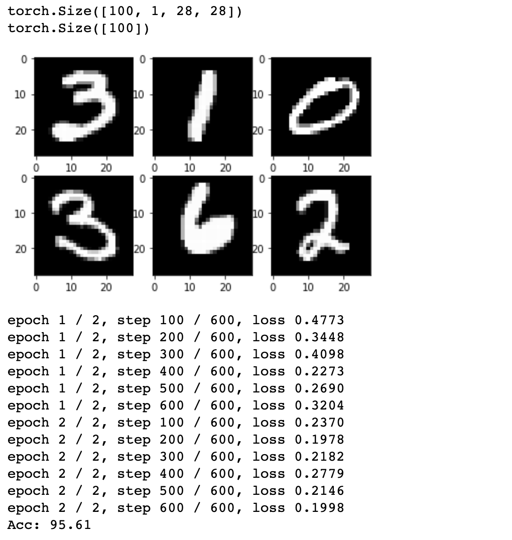
examples = iter(train_loader)
features, label = examples.next()
print(features.shape)
print(label.shape)
for i in range(6):
plt.subplot(2,3, i+1)
plt.imshow(features[i][0], cmap='gray')
plt.show()
# model
class NeuralNet(nn.Module):
def __init__(self, input_size, hidden_size, num_classes):
super(NeuralNet, self).__init__()
self.l1 = nn.Linear(input_size, hidden_size)
self.l2 = nn.Linear(hidden_size, num_classes)
def forward(self, x):
out = F.relu(self.l1(x))
out = self.l2(out)
return out
model = NeuralNet(input_size, hidden_size, num_classes)
# loss and optimizer
criterion = nn.CrossEntropyLoss()
optimizer = torch.optim.Adam(model.parameters(), lr=learning_rate)
# training loop
n_total_steps = len(train_loader)
for epoch in range(num_epochs):
for i, (images, label) in enumerate(train_loader):
# 100, 1, 28, 28
# 100, 784
images = images.reshape(-1, 28*28).to(device)
label = label.to(device)
# forward
outputs = model(images)
loss = criterion(outputs, label)
# backward
loss.backward()
optimizer.step()
optimizer.zero_grad()
if (i+1) % 100 ==0:
print(f'epoch {epoch+1} / {num_epochs}, step {i+1} / {n_total_steps}, loss {loss.item():.4f}')
# test
with torch.no_grad():
n_correct = 0
n_sample = 0
for images, label in test_loader:
images = images.reshape(-1, 28*28).to(device)
label = label.to(device)
outputs = model(images)
# print(outputs)
# value, index
_, prdiction = torch.max(outputs, 1)
n_correct += torch.sum(torch.eq(prdiction, label)).item()
n_sample += label.shape[0]
print(f'Acc: {100.0*n_correct / n_sample}')
运行结果:
9. Convolutional Neural Net(CNN)
这里我们通过构造CNN模型并对图片进行分类,采用“CIFAR10”数据集,然后自定义Model,调用“交叉熵损失函数”和“SGD”优化器来对模型训练,模型训练结束之后对分类器的分类准确率进行了测试。
实验代码如下:
2
3
4
5
6
7
8
9
10
11
12
13
14
15
16
17
18
19
20
21
22
23
24
25
26
27
28
29
30
31
32
33
34
35
36
37
38
39
40
41
42
43
44
45
46
47
48
49
50
51
52
53
54
55
56
57
58
59
60
61
62
63
64
65
66
67
68
69
70
71
72
73
74
75
76
77
78
79
80
81
82
83
84
85
86
87
88
89
90
91
92
93
94
95
96
97
98
99
100
101
102
103
104
105
106
107
108
109
110
111
112
113
114
115
116
117
import torch.nn as nn
import torchvision
import torchvision.transforms as transforms
import matplotlib.pyplot as plt
import numpy as np
import torch.nn.functional as F
# device config
device =torch.device('cuda' if torch.cuda.is_available() else 'cpu')
# hyper parameters
num_epochs = 4
batch_size = 4
learning_rate =0.001
# dataset has PILImage images of range[0,1]
# We transform them to Tensor of normalised range[-1, 1]
transform = transforms.Compose(
[
transforms.ToTensor(),
transforms.Normalize((0.5, 0.5, 0.5),(0.5, 0.5, 0.5))
]
)
train_dataset = torchvision.datasets.CIFAR10(root='./data', train=True,
download=True, transform=transform)
test_dataset = torchvision.datasets.CIFAR10(root='./data', train=False,
download=True, transform=transform)
train_loader = torch.utils.data.DataLoader(dataset=train_dataset, batch_size=batch_size,
shuffle=True)
test_loader = torch.utils.data.DataLoader(dataset=test_dataset, batch_size=batch_size,
shuffle=False)
classes =('plane', 'car','bird','cat','deer','dog','frog',
'horse','ship','truck')
def imshow(img):
img = img / 2 + 0.5 # unnormalize
npimg = img.numpy()
plt.imshow(np.transpose(npimg, (1, 2, 0)))
plt.show()
# model
class ConvNet(nn.Module):
def __init__(self):
super(ConvNet, self).__init__()
self.conv1 = nn.Conv2d(3,6,5)
self.pool = nn.MaxPool2d(2,2)
self.conv2 = nn.Conv2d(6,16,5)
self.fc1 = nn.Linear(16*5*5, 120)
self.fc2 = nn.Linear(120, 84)
self.fc3 = nn.Linear(84, 10)
def forward(self,x):
x = self.pool( F.relu(self.conv1(x)))
x = self.pool(F.relu(self.conv2(x)))
x = x.view(-1,16*5*5)
x = F.relu(self.fc1(x))
x = F.relu(self.fc2(x))
x = self.fc3(x)
return x
model = ConvNet().to(device)
criterion = nn.CrossEntropyLoss()
optimizer = torch.optim.SGD(model.parameters(), lr=learning_rate)
n_total_steps = len(train_loader)
for epoch in range(num_epochs):
for i,(images, labels) in enumerate(train_loader):
# origin shape:[4,3,32,32] = 4,3, 1024
# input_layer:3 input channels, 6 output channels, 5 kernel size
images = images.to(device)
labels = labels.to(device)
# Forward pass
outputs = model(images)
loss = criterion(outputs, labels)
# Backward and optimizer
optimizer.zero_grad()
loss.backward()
optimizer.step()
if (i+1) % 2000 == 0:
print(f'Epoch [{epoch+1}/{num_epochs}], Step [{i+1}/{n_total_steps}], Loss: {loss.item():.4f}')
# test
with torch.no_grad():
n_correct = 0
n_samples = 0
n_class_correct = [0 for i in range(10)]
n_class_samples = [0 for i in range(10)]
for images, labels in test_loader:
images = images.to(device)
labels = labels.to(device)
outputs = model(images)
# max returns (value ,index)
_, predicted = torch.max(outputs, 1)
n_samples += labels.size(0)
n_correct += (predicted == labels).sum().item()
for i in range(batch_size):
label = labels[i]
pred = predicted[i]
if (label == pred):
n_class_correct[label] += 1
n_class_samples[label] += 1
acc = 100.0 * n_correct / n_samples
print(f'Accuracy of the network: {acc} %')
for i in range(10):
acc = 100.0 * n_class_correct[i] / n_class_samples[i]
print(f'Accuracy of {classes[i]}: {acc} %')
10. Transfer Learning
这里我们学习迁移学习,主要学习如下三个知识点:
ImageFolder: how we can use ImageFolder
Scheduler: how we use a scheduler to change the learning rate
Transfer Learning
迁移学习是指在某一个任务上训练好模型,然后将训练好的模型迁移到另外一个任务中,固定模型的某些参数,对另外一些参数进行学习,以便模型能够适应新的任务。
实验代码如下:
2
3
4
5
6
7
8
9
10
11
12
13
14
15
16
17
18
19
20
21
22
23
24
25
26
27
28
29
30
31
32
33
34
35
36
37
38
39
40
41
42
43
44
45
46
47
48
49
50
51
52
53
54
55
56
57
58
59
60
61
62
63
64
65
66
67
68
69
70
71
72
73
74
75
76
77
78
79
80
81
82
83
84
85
86
87
88
89
90
91
92
93
94
95
96
97
98
99
100
101
102
103
104
105
106
107
108
109
110
111
112
113
114
115
116
117
118
119
120
121
122
123
124
125
126
127
128
129
130
131
132
133
134
135
136
137
138
139
140
141
142
143
144
145
146
147
148
149
150
151
152
# 1) ImageFolder: how we can use ImageFolder
# 2) Scheduler: how we use a scheduler to change the learning rate
# 3) Transfer Learning:
import torch
import torch.nn as nn
import torch.optim as optim
from torch.optim import lr_scheduler
import numpy as np
import torchvision
from torchvision import datasets, models, transforms
import matplotlib.pyplot as plt
import time
import os
import copy
# device config
device =torch.device('cuda' if torch.cuda.is_available() else 'cpu')
mean = np.array([0.485, 0.456, 0.406])
std = np.array([0.229, 0.224, 0.225])
data_transforms = {
'train':transforms.Compose([
transforms.RandomResizedCrop(224),
transforms.RandomHorizontalFlip(),
transforms.ToTensor(),
transforms.Normalize(mean, std)
]),
'val':transforms.Compose([
transforms.Resize(256),
transforms.CenterCrop(224),
transforms.ToTensor(),
transforms.Normalize(mean, std)
])
}
# import data
data_dir = 'data/hymenoptera_data'
sets = ['train', 'val']
image_datasets = {x:datasets.ImageFolder(os.path.join(data_dir, x),
data_transforms[x])
for x in sets}
dataloaders = {x: torch.utils.data.DataLoader(image_datasets[x], batch_size=4,
shuffle=True, num_workers=0)
for x in sets}
dataset_sizes = {x: len(image_datasets[x]) for x in sets}
class_names = image_datasets['train'].classes
print(class_names)
def imshow(inp, title):
"""Imshow for Tensor."""
inp = inp.numpy().transpose((1, 2, 0))
inp = std * inp + mean
inp = np.clip(inp, 0, 1)
plt.imshow(inp)
plt.title(title)
plt.show()
# Get a batch of training data
inputs, classes = next(iter(dataloaders['train']))
# Make a grid from batch
out = torchvision.utils.make_grid(inputs)
imshow(out, title=[class_names[x] for x in classes])
def train_model(model, criterion, optimizer, scheduler, num_epochs=25):
since = time.time()
best_model_wts = copy.deepcopy(model.state_dict())
best_acc = 0.0
for epoch in range(num_epochs):
print(f'Epoch {epoch+1} / {num_epochs}')
print('-'*15)
# Each epoch has a training and validation phase
for phase in sets:
if phase =='train':
model.train()
else:
model.eval()
running_loss = 0.0
running_correct = 0.0
# Iterate over data.
for inputs, labels in dataloaders[phase]:
inputs = inputs.to(device)
labels = labels.to(device)
# forward
# track history if only training
with torch.set_grad_enabled(phase == 'train'):
outputs = model(inputs)
loss = criterion(outputs, labels)
_, preds = torch.max(outputs, 1)
# backward + optimizer only if in training phase
if phase == 'train':
optimizer.zero_grad()
loss.backward()
optimizer.step()
# statistics
running_loss += loss.item()*inputs.size(0)
running_correct += torch.sum(preds == labels.data)
if phase == 'train':
scheduler.step()
epoch_loss = running_loss / dataset_sizes[phase]
epoch_acc = running_correct.double() / dataset_sizes[phase]
print(f'{phase} Loss: {epoch_loss:.4f} Acc: {epoch_acc:.4f}')
# deep copy the model to
if phase == 'val' and epoch_acc > best_acc:
best_acc = epoch_acc
best_model_wts = copy.deepcopy(model.state_dict())
time_elapsed = time.time()-since
print(f'Training complete in {time_elapsed//60:.0f}m {time_elapsed%60:.0fs}')
print(f'Best val Acc: {best_acc:4f}')
#load best model weights
model.load_state_dic(best_model_wts)
return model
model = models.resnet18(pretrained=True)
# Here, we need to freeze all the network except the final layer.
# We need to set requires_grad == False to freeze the parameters so that the gradients are not computed in backward()
for param in model.parameters():
param.requires_grad = False
num_ftrs = model.fc.in_features
model.fc = nn.Linear(num_ftrs, 2)
model.to(device)
criterion = nn.CrossEntropyLoss()
# Observe that all parameters are being optimized
optimizer = optim.SGD(model.parameters(), lr=0.001)
# scheduler
step_lr_schedule = lr_scheduler.StepLR(optimizer, step_size=7, gamma=0.1) # Every 7 step, learning rate multiple by 0.1
model = train_model(model, criterion, optimizer, step_lr_schedule, num_epochs=7)
11. Tensorboard
Tensorbard是很好的可视化工具,具体可以参考如下的代码。
2
3
4
5
6
7
8
9
10
11
12
13
14
15
16
17
18
19
20
21
22
23
24
25
26
27
28
29
30
31
32
33
34
35
36
37
38
39
40
41
42
43
44
45
46
47
48
49
50
51
52
53
54
55
56
57
58
59
60
61
62
63
64
65
66
67
68
69
70
71
72
73
74
75
76
77
78
79
80
81
82
83
84
85
86
87
88
89
90
91
92
93
94
95
96
97
98
99
100
101
102
103
104
105
106
107
108
109
110
111
112
113
114
115
116
117
118
119
120
121
122
123
124
125
126
127
128
129
130
131
132
133
134
135
136
137
138
139
140
141
142
143
144
145
146
147
148
149
150
151
152
153
154
155
156
157
158
159
160
161
162
163
164
165
import torch
import torch.nn as nn
import torchvision
import torchvision.transforms as transforms
import matplotlib.pyplot as plt
############## TENSORBOARD ########################
import sys
import torch.nn.functional as F
from torch.utils.tensorboard import SummaryWriter
# default `log_dir` is "runs" - we'll be more specific here
writer = SummaryWriter('runs/mnist1')
###################################################
# Device configuration
device = torch.device('cuda' if torch.cuda.is_available() else 'cpu')
# Hyper-parameters
input_size = 784 # 28x28
hidden_size = 500
num_classes = 10
num_epochs = 1
batch_size = 64
learning_rate = 0.001
# MNIST dataset
train_dataset = torchvision.datasets.MNIST(root='./data',
train=True,
transform=transforms.ToTensor(),
download=True)
test_dataset = torchvision.datasets.MNIST(root='./data',
train=False,
transform=transforms.ToTensor())
# Data loader
train_loader = torch.utils.data.DataLoader(dataset=train_dataset,
batch_size=batch_size,
shuffle=True)
test_loader = torch.utils.data.DataLoader(dataset=test_dataset,
batch_size=batch_size,
shuffle=False)
examples = iter(test_loader)
example_data, example_targets = examples.next()
for i in range(6):
plt.subplot(2, 3, i + 1)
plt.imshow(example_data[i][0], cmap='gray')
# plt.show()
############## TENSORBOARD ########################
img_grid = torchvision.utils.make_grid(example_data)
writer.add_image('mnist_images', img_grid)
# writer.close()
# sys.exit()
###################################################
# Fully connected neural network with one hidden layer
class NeuralNet(nn.Module):
def __init__(self, input_size, hidden_size, num_classes):
super(NeuralNet, self).__init__()
self.input_size = input_size
self.l1 = nn.Linear(input_size, hidden_size)
self.relu = nn.ReLU()
self.l2 = nn.Linear(hidden_size, num_classes)
def forward(self, x):
out = self.l1(x)
out = self.relu(out)
out = self.l2(out)
# no activation and no softmax at the end
return out
model = NeuralNet(input_size, hidden_size, num_classes).to(device)
# Loss and optimizer
criterion = nn.CrossEntropyLoss()
optimizer = torch.optim.Adam(model.parameters(), lr=learning_rate)
############## TENSORBOARD ########################
writer.add_graph(model, example_data.reshape(-1, 28 * 28))
# writer.close()
# sys.exit()
###################################################
# Train the model
running_loss = 0.0
running_correct = 0
n_total_steps = len(train_loader)
for epoch in range(num_epochs):
for i, (images, labels) in enumerate(train_loader):
# origin shape: [100, 1, 28, 28]
# resized: [100, 784]
images = images.reshape(-1, 28 * 28).to(device)
labels = labels.to(device)
# Forward pass
outputs = model(images)
loss = criterion(outputs, labels)
# Backward and optimize
optimizer.zero_grad()
loss.backward()
optimizer.step()
running_loss += loss.item()
_, predicted = torch.max(outputs.data, 1)
running_correct += (predicted == labels).sum().item()
if (i + 1) % 100 == 0:
print(f'Epoch [{epoch + 1}/{num_epochs}], Step [{i + 1}/{n_total_steps}], Loss: {loss.item():.4f}')
############## TENSORBOARD ########################
writer.add_scalar('training loss', running_loss / 100, epoch * n_total_steps + i)
running_accuracy = running_correct / 100 / predicted.size(0)
writer.add_scalar('accuracy', running_accuracy, epoch * n_total_steps + i)
running_correct = 0
running_loss = 0.0
###################################################
# Test the model
# In test phase, we don't need to compute gradients (for memory efficiency)
class_labels = []
class_preds = []
with torch.no_grad():
n_correct = 0
n_samples = 0
for images, labels in test_loader:
images = images.reshape(-1, 28 * 28).to(device)
labels = labels.to(device)
outputs = model(images)
# max returns (value ,index)
values, predicted = torch.max(outputs.data, 1)
n_samples += labels.size(0)
n_correct += (predicted == labels).sum().item()
class_probs_batch = [F.softmax(output, dim=0) for output in outputs]
class_preds.append(class_probs_batch)
class_labels.append(predicted)
# 10000, 10, and 10000, 1
# stack concatenates tensors along a new dimension
# cat concatenates tensors in the given dimension
class_preds = torch.cat([torch.stack(batch) for batch in class_preds])
class_labels = torch.cat(class_labels)
acc = 100.0 * n_correct / n_samples
print(f'Accuracy of the network on the 10000 test images: {acc} %')
############## TENSORBOARD ########################
classes = range(10)
for i in classes:
labels_i = class_labels == i
preds_i = class_preds[:, i]
writer.add_pr_curve(str(i), labels_i, preds_i, global_step=0)
writer.close()
###################################################
12. Saving and Loading model
2
3
4
5
6
7
8
9
10
11
12
13
14
15
16
2 DIFFERENT WAYS OF SAVING
# 1) lazy way: save whole model
torch.save(model, PATH)

# model class must be defined somewhere
model = torch.load(PATH)
model.eval()

# 2) recommended way: save only the state_dict
torch.save(model.state_dict(), PATH)

# model must be created again with parameters
model = Model(*args, **kwargs)
model.load_state_dict(torch.load(PATH))
model.eval()
示例代码如下:
2
3
4
5
6
7
8
9
10
11
12
13
14
15
16
17
18
19
20
21
22
23
24
25
26
27
28
29
30
31
32
33
34
35
36
37
38
39
40
41
42
43
44
45
46
47
48
49
50
51
52
53
54
55
56
57
58
59
60
61
62
63
64
65
66
67
68
69
70
71
72
73
74
75
76
77
78
79
80
81
82
83
84
85
86
87
88
89
90
91
92
93
94
95
96
97
98
99
100
101
102
103
104
105
106
107
108
109
110
111
import torch.nn as nn
class Model(nn.Module):
def __init__(self, n_input_features):
super(Model, self).__init__()
self.linear = nn.Linear(n_input_features, 1)
def forward(self, x):
y_pred = torch.sigmoid(self.linear(x))
return y_pred
model = Model(n_input_features=6)
# train your model...
####################save all ######################################
for param in model.parameters():
print(param)
# save and load entire model
FILE = "model.pth"
torch.save(model, FILE)
loaded_model = torch.load(FILE)
loaded_model.eval()
for param in loaded_model.parameters():
print(param)
############save only state dict #########################
# save only state dict
FILE = "model.pth"
torch.save(model.state_dict(), FILE)
print(model.state_dict())
loaded_model = Model(n_input_features=6)
loaded_model.load_state_dict(torch.load(FILE)) # it takes the loaded dictionary, not the path file itself
loaded_model.eval()
print(loaded_model.state_dict())
###########load checkpoint#####################
learning_rate = 0.01
optimizer = torch.optim.SGD(model.parameters(), lr=learning_rate)
checkpoint = {
"epoch": 90,
"model_state": model.state_dict(),
"optim_state": optimizer.state_dict()
}
print(optimizer.state_dict())
FILE = "checkpoint.pth"
torch.save(checkpoint, FILE)
model = Model(n_input_features=6)
optimizer = optimizer = torch.optim.SGD(model.parameters(), lr=0)
checkpoint = torch.load(FILE)
model.load_state_dict(checkpoint['model_state'])
optimizer.load_state_dict(checkpoint['optim_state'])
epoch = checkpoint['epoch']
model.eval()
# - or -
# model.train()
print(optimizer.state_dict())
# Remember that you must call model.eval() to set dropout and batch normalization layers
# to evaluation mode before running inference. Failing to do this will yield
# inconsistent inference results. If you wish to resuming training,
# call model.train() to ensure these layers are in training mode.
""" SAVING ON GPU/CPU
# 1) Save on GPU, Load on CPU
device = torch.device("cuda")
model.to(device)
torch.save(model.state_dict(), PATH)
device = torch.device('cpu')
model = Model(*args, **kwargs)
model.load_state_dict(torch.load(PATH, map_location=device))
# 2) Save on GPU, Load on GPU
device = torch.device("cuda")
model.to(device)
torch.save(model.state_dict(), PATH)
model = Model(*args, **kwargs)
model.load_state_dict(torch.load(PATH))
model.to(device)
# Note: Be sure to use the .to(torch.device('cuda')) function
# on all model inputs, too!
# 3) Save on CPU, Load on GPU
torch.save(model.state_dict(), PATH)
device = torch.device("cuda")
model = Model(*args, **kwargs)
model.load_state_dict(torch.load(PATH, map_location="cuda:0")) # Choose whatever GPU device number you want
model.to(device)
# This loads the model to a given GPU device.
# Next, be sure to call model.to(torch.device('cuda')) to convert the model’s parameter tensors to CUDA tensors
"""
13. Summary